Sampling, the Central Limit Theorem and Confidence Intervals

Almost every business number is an estimate. When you say "the average basket is ₹659" you are usually describing a sample: this year's orders, one city's customers or a survey of 200 people, and hoping it represents a larger population: every order the company will ever get. A different sample would have given a slightly different number. Statistical inference is the toolkit for saying how far off your estimate might be.

In this lesson you will draw random samples with pandas and NumPy, watch the sampling distribution of the mean take shape, see why the central limit theorem makes the normal curve so useful, and compute confidence intervals: ranges that express the uncertainty of an estimate. We cover the classic formula for a mean, the interval for a proportion (such as the cancellation rate), and the flexible bootstrap, which works for almost any statistic, including the median.

Treat the 6,000 FreshBasket orders as our "population" for the first experiments, because then we can compare each sample estimate with the true answer, something you can never do in real life.

Worked examples

Example 1: Population and sample

Question: How close is the mean of a small sample to the true mean?

import pandas as pd
import numpy as np

items = pd.read_csv("order_items.csv")
population = (items["quantity"] * items["unit_price"]).groupby(items["order_id"]).sum()

print("population size :", len(population))
print("true mean       :", round(population.mean(), 2))

sample = population.sample(100, random_state=42)
print("sample mean (100):", round(sample.mean(), 2))
print("error            :", round(sample.mean() - population.mean(), 2))

population size : 6000
true mean       : 659.23
sample mean (100): 702.45
error            : 43.22

How it works: The population mean is a fixed number (a parameter). The sample mean is a statistic: it varies from sample to sample. sample(n, random_state=...) draws a simple random sample without replacement; fixing the seed makes the result reproducible. A random sample is representative on average, but any single sample has some error.

Reading the result: The true mean order value is ₹659.23 and the 100-order sample gives ₹702.45, an error of ₹43.22. A different seed would give a different error.

Example 2: The sampling distribution

Question: How much do sample means vary if we repeat the sampling many times?

rng = np.random.default_rng(0)
means_100 = np.array([rng.choice(population.values, 100, replace=False).mean() for _ in range(2000)])

print("average of 2000 sample means:", round(means_100.mean(), 2))
print("spread (std) of sample means :", round(means_100.std(), 2))
print("min / max sample mean        :", round(means_100.min(), 1), round(means_100.max(), 1))

average of 2000 sample means: 657.06
spread (std) of sample means : 48.54
min / max sample mean        : 501.6 813.5

How it works: We drew 2,000 different samples of 100 orders and recorded each sample's mean. That collection is the sampling distribution of the mean. Two facts matter: it is centred on the true mean (sampling is unbiased), and its standard deviation (the standard error) tells us the typical size of the sampling error.

Reading the result: The 2,000 sample means average ₹657.06, almost exactly the true ₹659.23. Their standard deviation, the standard error, is ₹48.54, so a typical 100-order sample misses by about that much.

Example 3: The standard error formula

Question: Can we compute the standard error without repeating the experiment?

n = 100
sigma = population.std()
se_formula = sigma / np.sqrt(n)
print("formula  sigma/sqrt(n):", round(se_formula, 2))
print("simulated            :", round(means_100.std(), 2))

# from a single sample (what you can do in real life)
se_one = sample.std(ddof=1) / np.sqrt(len(sample))
print("from one sample      :", round(se_one, 2))

for n in (25, 100, 400, 1600):
    print(n, round(sigma / np.sqrt(n), 1))

formula  sigma/sqrt(n): 49.93
simulated            : 48.54
from one sample      : 49.11
25 99.9
100 49.9
400 25.0
1600 12.5

How it works: The standard error of the mean is the data's standard deviation divided by the square root of the sample size. You only need one sample: estimate the standard deviation from it. The square root has a practical consequence: to halve the error you need four times the data, and to cut it by a factor of ten you need a hundred times as much.

Reading the result: The formula gives ₹49.93 and the simulation ₹48.54, which agree closely (the small gap comes from simulation noise and from the fact that we sample without replacement from a finite pool). A single 100-order sample estimates it as ₹49.11.

Example 4: The central limit theorem

Question: Order values are skewed. Are their averages skewed too?

import matplotlib.pyplot as plt
import skillancy_style
from scipy import stats

rng = np.random.default_rng(1)
fig, axes = plt.subplots(1, 4, figsize=(13, 3.4), sharey=False)
sizes = [1, 5, 30, 200]
skews = {}
for ax, n_ in zip(axes, sizes):
    m = np.array([rng.choice(population.values, n_).mean() for _ in range(3000)])
    skews[n_] = stats.skew(m)
    ax.hist(m, bins=40, color="#028090", edgecolor="white")
    ax.set_title(f"n = {n_}", loc="left")
    ax.set_xlabel("Sample mean (₹)")
fig.suptitle("Averages become bell-shaped as the sample grows", x=0.01, y=1.08, ha="left", fontweight="bold")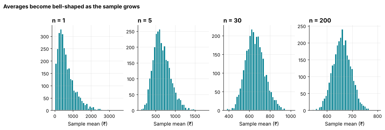

How it works: The central limit theorem says that the mean of many independent observations is approximately normally distributed, whatever the shape of the original data, as long as the sample is reasonably large. With n = 1 we see the skewed raw data; by n = 30 the distribution of means is already close to symmetric and by n = 200 it is a narrow bell. This is why normal-based methods work on money, durations and counts.

Reading the result: The skewness of the sample means falls from 1.63 at n = 1 to 0.69 at n = 5, 0.28 at n = 30 and 0.09 at n = 200, while the spread shrinks steadily.

Example 5: A confidence interval for a mean

Question: What range is plausible for the true average basket, given a sample of 100?

m = sample.mean()
se = sample.std(ddof=1) / np.sqrt(len(sample))
t_crit = stats.t.ppf(0.975, df=len(sample) - 1)
low, high = m - t_crit * se, m + t_crit * se
print("t critical value:", round(t_crit, 3))
print("95% CI:", round(low, 1), "to", round(high, 1))

print(stats.t.interval(0.95, df=len(sample) - 1, loc=m, scale=se))
print("contains true mean:", low <= population.mean() <= high)

t critical value: 1.984
95% CI: 605.0 to 799.9
(np.float64(605.0099194408361), np.float64(799.890080559164))
contains true mean: True

How it works: A 95% confidence interval for the mean is the sample mean plus or minus about two standard errors; the exact multiplier is the t critical value, which is slightly above 1.96 for small samples. stats.t.interval does the same in one call. The interval is the estimate with an honest margin of error attached.

Reading the result: From 100 orders we estimate the average basket at ₹702.5 with a 95% confidence interval of ₹605 to ₹800. The true mean (₹659) falls inside.

Example 6: What "95% confidence" really means

Question: If we repeat this process, how often does the interval catch the true mean?

rng = np.random.default_rng(5)
hits = 0
trials = 1000
widths = []
for _ in range(trials):
    s_ = rng.choice(population.values, 100, replace=False)
    se_ = s_.std(ddof=1) / np.sqrt(100)
    t_ = stats.t.ppf(0.975, 99)
    lo_, hi_ = s_.mean() - t_ * se_, s_.mean() + t_ * se_
    hits += lo_ <= population.mean() <= hi_
    widths.append(hi_ - lo_)

print("coverage:", hits / trials)
print("average width:", round(np.mean(widths), 1))

coverage: 0.945
average width: 196.8

How it works: The "95%" describes the procedure, not one particular interval. If you repeated the sampling many times and built an interval each time, about 95% of the intervals would contain the true mean. Any single interval either contains it or does not; we just do not know which. It is not correct to say "there is a 95% probability that the true mean is in this interval".

Reading the result: 945 of 1000 intervals (94.5%) covered the true mean, close to the nominal 95%. The average width was ₹197.

Example 7: Sample size and precision

Question: How does the interval shrink as the sample grows?

rng = np.random.default_rng(8)
rows = []
for n_ in (25, 100, 400, 1600):
    s_ = pd.Series(rng.choice(population.values, n_, replace=False))
    lo_, hi_ = stats.t.interval(0.95, df=n_ - 1, loc=s_.mean(), scale=s_.sem())
    rows.append({"n": n_, "mean": s_.mean(), "margin": (hi_ - lo_) / 2})
ci_table = pd.DataFrame(rows).round(1)
print(ci_table)
print(round(ci_table["margin"].iloc[0] / ci_table["margin"].iloc[-1], 1))

      n   mean  margin
0    25  638.5   209.8
1   100  573.1    92.1
2   400  654.9    46.4
3  1600  668.6    24.7
8.5

How it works: Series.sem() returns the standard error of the mean directly. The margin of error is half the interval width. Because the standard error shrinks with the square root of n, going from 25 to 1,600 orders (64 times more data) reduces the margin only by about eight times. Precision gets more expensive as you ask for more of it.

Reading the result: The margin of error falls from ₹210 at n = 25 to ₹25 at n = 1,600, a reduction of 8.5 times.

Example 8: A confidence interval for a proportion

Question: What is the plausible range for the cancellation rate?

orders = pd.read_csv("orders.csv", parse_dates=["order_date"])
n_orders = len(orders)
cancelled = int((orders["order_status"] == "Cancelled").sum())
p_hat = cancelled / n_orders

se_p = np.sqrt(p_hat * (1 - p_hat) / n_orders)
wald = (p_hat - 1.96 * se_p, p_hat + 1.96 * se_p)
wilson = stats.binomtest(cancelled, n_orders).proportion_ci(confidence_level=0.95, method="wilson")

print("cancellation rate:", round(p_hat, 4))
print("Wald  :", tuple(round(x, 4) for x in wald))
print("Wilson:", round(wilson.low, 4), round(wilson.high, 4))

cancellation rate: 0.0617
Wald  : (np.float64(0.0556), np.float64(0.0678))
Wilson: 0.0559 0.068

How it works: A proportion's standard error is the square root of p(1-p)/n. The simple "Wald" interval uses it directly; the Wilson interval (available through binomtest(...).proportion_ci) behaves better for small samples or rates near 0 or 1. With 6,000 orders and a rate near 6%, they are practically the same.

Reading the result: 370 of 6000 orders were cancelled: 6.17%, with a 95% interval of 5.59% to 6.80%. A change from 6.2% to 6.4% next month would be well within the noise.

Example 9: The bootstrap for a median

Question: What is the uncertainty on the median order value, which has no simple formula?

rng = np.random.default_rng(21)
boot_medians = np.array([
    np.median(rng.choice(sample.values, size=len(sample), replace=True))
    for _ in range(5000)
])
ci = np.percentile(boot_medians, [2.5, 97.5])

print("sample median      :", round(sample.median(), 1))
print("bootstrap 95% CI   :", ci.round(1))
print("true median        :", round(population.median(), 1))

sample median      : 653.0
bootstrap 95% CI   : [465. 774.]
true median        : 536.0

How it works: The bootstrap treats the sample as a stand-in for the population: resample it with replacement many times, compute the statistic each time, and use the spread of those results as the uncertainty. The 2.5th and 97.5th percentiles of the bootstrap statistics form a 95% interval. It needs no formula, so it works for medians, percentiles, ratios and other awkward statistics.

Reading the result: The sample median is ₹653 and the bootstrap interval runs from ₹465 to ₹774. The true median of ₹536 lies inside it.

Example 10: How big a sample do I need?

Question: How many orders must we survey to estimate the average basket to within ±₹20?

margin = 20
sigma_est = sample.std(ddof=1)
n_needed = int(np.ceil((1.96 * sigma_est / margin) ** 2))
print("estimated sigma:", round(sigma_est, 1))
print("sample size needed:", n_needed)

# for a proportion: margin of +/-2 points, worst case p = 0.5
n_prop = int(np.ceil(1.96 ** 2 * 0.25 / 0.02 ** 2))
print("poll size for +/-2 points:", n_prop)

estimated sigma: 491.1
sample size needed: 2317
poll size for +/-2 points: 2401

How it works: Rearranging the margin-of-error formula (margin = 1.96 x sigma / sqrt(n)) gives n = (1.96 x sigma / margin)^2. You need an estimate of sigma, from a pilot sample or past data. For polls and rates, the worst case is p = 0.5, which gives the famous result that about 2,400 respondents give roughly plus or minus two percentage points.

Reading the result: To estimate the average basket within ±₹20 we need about 2317 orders. A rate estimated to ±2 percentage points needs 2401 observations in the worst case.

Common mistakes

1. Reading "95% confidence" as "95% chance the true value is inside this interval". It describes the long-run behaviour of the method.

2. Confusing the standard deviation with the standard error. One describes the data, the other the precision of an estimate.

3. Sampling a convenient subset (the first rows, one city) instead of a random one. Sampling bias cannot be fixed with a bigger sample.

4. Bootstrapping with replace=False, which just reproduces the sample.

5. Assuming normality with tiny samples from heavily skewed data, where the central limit theorem has not kicked in.

population.sample(10000)

Traceback (most recent call last):
  File "example.py", line 1, in <module>
    population.sample(10000)
    ~~~~~~~~~~~~~~~~~^^^^^^^
  File "example.py", line 5988, in sample
    sampled_indices = sample.sample(obj_len, size, replace, weights, rs)
  File "example.py", line 161, in sample
    return random_state.choice(obj_len, size=size, replace=replace, p=weights).astype(
           ~~~~~~~~~~~~~~~~~~~^^^^^^^^^^^^^^^^^^^^^^^^^^^^^^^^^^^^^^^^^^^^^^^^
  File "example.py", line 1025, in numpy.random.mtrand.RandomState.choice
ValueError: Cannot take a larger sample than population when 'replace=False'

Practice questions

Practice 1 (Easy): Standard error of delivery time

Compute the mean delivery time and its standard error for all delivered orders.

mins = orders["delivery_minutes"].dropna()
print(round(mins.mean(), 3), round(mins.sem(), 3))

23.67 0.092

Practice 2 (Medium): 99% interval

Compute a 99% confidence interval for the mean delivery time and compare its width with the 95% interval.

ci95 = stats.t.interval(0.95, df=len(mins) - 1, loc=mins.mean(), scale=mins.sem())
ci99 = stats.t.interval(0.99, df=len(mins) - 1, loc=mins.mean(), scale=mins.sem())
print(np.round(ci95, 3), np.round(ci99, 3))
print(round((ci99[1] - ci99[0]) / (ci95[1] - ci95[0]), 2))

[23.489 23.851] [23.432 23.908]
1.31

Practice 3 (Hard): Bootstrap the 90th percentile

Bootstrap a 95% interval for the 90th percentile of delivery minutes, using 2,000 resamples of the full delivered data.

rng = np.random.default_rng(99)
vals = mins.values
boot_p90 = np.array([np.percentile(rng.choice(vals, len(vals), replace=True), 90) for _ in range(2000)])
lo90, hi90 = np.percentile(boot_p90, [2.5, 97.5])
print(np.percentile(vals, 90), round(lo90, 2), round(hi90, 2))

32.0 32.0 33.0

Key takeaways

• A statistic varies from sample to sample; the standard error (sd / sqrt(n)) measures by how much.
• The central limit theorem makes sample means approximately normal for large enough samples, whatever the raw shape.
• A 95% confidence interval is estimate ± about two standard errors; the 95% describes the method's long-run coverage.
• To halve the margin of error you need four times the data.
• Proportions have their own interval (Wilson is a safe choice).
• The bootstrap gives an interval for almost any statistic by resampling with replacement.
• Random sampling beats big sampling: size cannot cure bias.