Case Study: Explaining Revenue Growth, Step by Step

So far we have learned tools one at a time. Real analysis starts differently: someone asks a messy question and you must choose the tools yourself. This lesson is a complete case study that works like a real request.

The founder asks: "Revenue has grown enormously since January 2025. What actually drove it, and is it still growing?"

A good analyst does not run random charts. They (1) turn the question into measurable parts, (2) check the data, (3) decompose the number into drivers, (4) look for the story behind the biggest driver, (5) test the finding from a second angle and (6) write it down plainly. We will follow exactly those steps using FreshBasket data, and use the techniques from this module: groupby, indexing to a base period, growth rates, cohorts, charts and generated text.

The answer has a twist. The headline number tells one story, but one extra cut of the data reveals something the founder may not want to hear. Finding that twist is the difference between reporting numbers and doing analysis.

Worked examples

Example 1: Break the question into a metric tree

Question: What is revenue made of?

import pandas as pd
import numpy as np

orders = pd.read_csv("orders.csv", parse_dates=["order_date"])
items = pd.read_csv("order_items.csv")
customers = pd.read_csv("customers.csv", parse_dates=["signup_date"])

value = (items["quantity"] * items["unit_price"]).groupby(items["order_id"]).sum().rename("value")
d = orders.merge(value, on="order_id")
d = d[d["order_status"] == "Delivered"].copy()
d["month"] = d["order_date"].dt.to_period("M")

monthly = d.groupby("month").agg(revenue=("value", "sum"), orders=("order_id", "count"), active=("customer_id", "nunique"))
monthly["orders_per_active"] = monthly["orders"] / monthly["active"]
monthly["aov"] = monthly["revenue"] / monthly["orders"]

check = monthly["active"] * monthly["orders_per_active"] * monthly["aov"]
print(np.allclose(check, monthly["revenue"]))
print(monthly.round(1).iloc[[0, 6, 12, -1]])

True
          revenue  orders  active  orders_per_active    aov
month                                                      
2025-01   32635.0      55      41                1.3  593.4
2025-07  123213.0     181     112                1.6  680.7
2026-01  263691.0     400     232                1.7  659.2
2026-06  388871.0     562     289                1.9  691.9

How it works: Revenue can be written as an identity: active customers x orders per active customer x average order value (AOV). Each factor is something a different team controls: marketing grows the customer base, retention and product grow frequency, merchandising and pricing grow basket size. The allclose check proves the three factors multiply back to revenue exactly, so no growth is "lost". We count delivered orders only, since cancelled and returned orders earn nothing.

Reading the result: Revenue per month rose from ₹32,635 in 2025-01 to ₹388,871 in 2026-06. We have 18 months of data to explain.

Example 2: Index the drivers to a base period

Question: Which driver grew the most?

base = monthly.iloc[0]
indexed = (monthly[["revenue", "active", "orders_per_active", "aov"]] / base[["revenue", "active", "orders_per_active", "aov"]] * 100).round(0)
print(indexed.iloc[[0, 5, 11, 17]])
print("multiples (last / first):")
print((monthly.iloc[-1][["revenue", "active", "orders_per_active", "aov"]] / base[["revenue", "active", "orders_per_active", "aov"]]).round(2))

         revenue  active  orders_per_active    aov
month                                             
2025-01    100.0   100.0              100.0  100.0
2025-06    341.0   249.0              124.0  111.0
2025-12    723.0   498.0              137.0  106.0
2026-06   1192.0   705.0              145.0  117.0
multiples (last / first):
revenue              11.92
active                7.05
orders_per_active     1.45
aov                   1.17
dtype: float64

How it works: Dividing each column by its first value and multiplying by 100 puts every series on the same scale (the base month equals 100), so a factor that grew 7x can be compared with one that grew 1.2x even though their raw units differ. This is the standard way to compare growth fairly.

Reading the result: Revenue is now 11.9 times its starting level. Active customers grew 7.0 times, orders per customer 1.45 times and the average order value only 1.17 times.

Example 3: Chart the three drivers

Question: Show the story visually.

import matplotlib.pyplot as plt
import skillancy_style

x = monthly.index.to_timestamp()
fig, ax = plt.subplots(figsize=(9.5, 4.4))
ax.plot(x, indexed["active"], color="#028090", linewidth=2.6, label="Active customers")
ax.plot(x, indexed["orders_per_active"], color="#F4A261", linewidth=2.6, label="Orders per customer")
ax.plot(x, indexed["aov"], color="#8D99AE", linewidth=2.6, label="Average order value")
ax.axhline(100, color="#264653", linewidth=1, linestyle=":")
ax.set_ylabel(f"Index ({monthly.index[0]} = 100)")
ax.set_title("More customers, not bigger baskets, drove growth", loc="left")
ax.legend(frameon=False, loc="upper left")
fig.autofmt_xdate()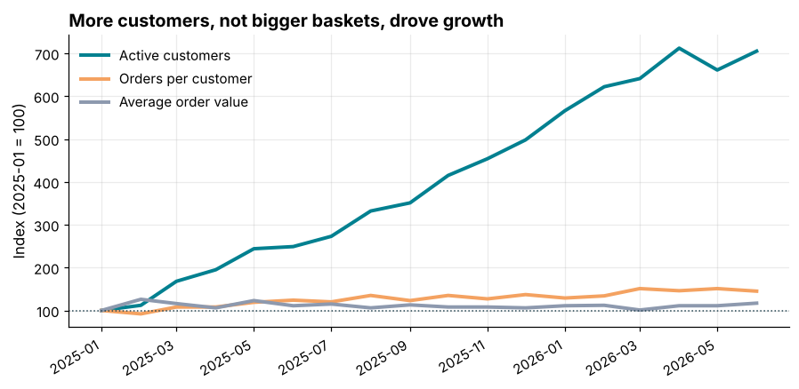

How it works: Three lines on one indexed scale make the ranking obvious: the line that climbs steeply is the main driver, and the flat one is irrelevant. The dotted line at 100 marks "no change". The title states the finding so the reader does not have to work it out.

Reading the result: The active-customer line climbs far above the others, ending near 705, while average order value stays within a narrow band around 111.

Example 4: Quantify each driver's contribution

Question: What share of the growth belongs to each factor?

logs = np.log(monthly[["active", "orders_per_active", "aov"]].iloc[-1] / monthly[["active", "orders_per_active", "aov"]].iloc[0])
total_log = np.log(monthly["revenue"].iloc[-1] / monthly["revenue"].iloc[0])
share = logs / total_log

print(share.round(3))
print("sum of shares:", round(share.sum(), 6))

active               0.788
orders_per_active    0.150
aov                  0.062
dtype: float64
sum of shares: 1.0

How it works: Because revenue is a product of three factors, the logarithm of the revenue growth is the sum of the logarithms of each factor's growth. Dividing each log by the total gives a clean additive split into percentage contributions that always adds to 100%. (A simple percentage split does not add up, because percentage changes multiply.)

Reading the result: Of the growth in revenue, 79% comes from having more active customers, 15% from each customer ordering more often and 6% from bigger baskets. Customer count is by far the dominant driver.

Example 5: New versus returning customers

Question: Is growth coming from acquiring people or from people coming back?

first_month = d.groupby("customer_id")["month"].min().rename("first_month")
d = d.merge(first_month, on="customer_id")
d["kind"] = np.where(d["month"] == d["first_month"], "New", "Returning")

mix = d.groupby(["month", "kind"])["order_id"].count().unstack(fill_value=0)
mix["new_share"] = mix["New"] / (mix["New"] + mix["Returning"])
print(mix.iloc[[1, 6, 11, 14, 15, 16, 17]])

kind     New  Returning  new_share
month                             
2025-02   33         24   0.578947
2025-07   54        127   0.298343
2025-12   53        321   0.141711
2026-03   33        500   0.061914
2026-04    9        561   0.015789
2026-05    4        544   0.007299
2026-06    4        558   0.007117

How it works: A customer's "first month" is the month of their first delivered order. Every order in that month counts as new-customer business; every later order is returning. Splitting the orders this way separates acquisition from retention, which are different problems with different fixes.

Reading the result: In 2025-07 new customers made 54 of the month's 181 orders, but in 2026-06 only 4 of 562. New customers have almost vanished from the recent months.

Example 6: Chart the acquisition cliff

Question: Show new and returning orders over time.

fig, ax = plt.subplots(figsize=(9.5, 4.4))
xm = mix.index.to_timestamp()
ax.bar(xm, mix["Returning"], width=22, color="#028090", label="Returning customers")
ax.bar(xm, mix["New"], width=22, bottom=mix["Returning"], color="#E76F51", label="New customers")
ax.set_ylabel("Delivered orders")
ax.set_title("New-customer orders have almost disappeared since March 2026", loc="left")
ax.legend(frameon=False, loc="upper left")
fig.autofmt_xdate()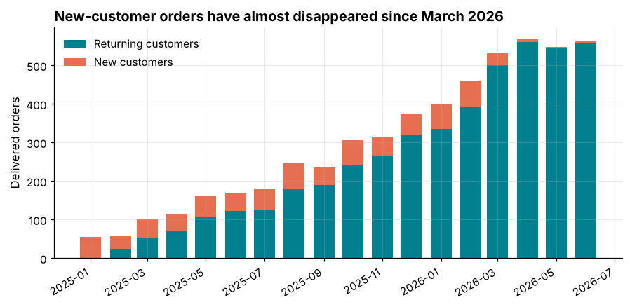

How it works: A stacked bar shows both the total and the mix at once. Returning-customer orders (teal) keep climbing while the coral new-customer slice stays roughly constant for a year and then collapses at the end. A title that names the date of the change focuses the reader on it.

Reading the result: New-customer orders were steady at about 55 per month from March 2025 to February 2026 but fell to 6 per month in the last three months.

Example 7: Find the cause in a second data source

Question: Why did new customers stop arriving?

signups = customers.groupby(customers["signup_date"].dt.to_period("M")).size()
print(signups.tail(6))
print("last signup date:", customers["signup_date"].max().date())
print("last data date  :", orders["order_date"].max().date())
print("gap (days):", (orders["order_date"].max() - customers["signup_date"].max()).days)

signup_date
2025-09    30
2025-10    39
2025-11    33
2025-12    23
2026-01    36
2026-02    19
Freq: M, dtype: int64
last signup date: 2026-02-19
last data date  : 2026-06-30
gap (days): 131

How it works: When one table shows a surprising change, look for the cause in another. The customer table records signup dates: if signups stopped, the first-order flow stops too. Joining ideas across tables (orders, customers, stores) is how an analyst moves from "what happened" to "why".

Reading the result: The last customer signed up on 2026-02-19, about 131 days before the end of the order data. The slowdown in new-customer orders follows the end of signups, so acquisition is the likely cause. Delivery quality is an unlikely explanation, because delivery times stayed flat throughout.

Example 8: Is growth still happening?

Question: What do recent growth rates say?

monthly["mom"] = monthly["revenue"].pct_change()
monthly["rolling3"] = monthly["revenue"].rolling(3).mean()
recent = monthly[["revenue", "mom"]].tail(6).copy()
recent["mom"] = (recent["mom"] * 100).round(1)
print(recent)

cagr_months = len(monthly) - 1
monthly_growth = (monthly["revenue"].iloc[-1] / monthly["revenue"].iloc[0]) ** (1 / cagr_months) - 1
print("average monthly growth over the whole period:", round(monthly_growth * 100, 1), "%")
print("average monthly growth, last 3 months:", round(((monthly["revenue"].iloc[-1] / monthly["revenue"].iloc[-4]) ** (1 / 3) - 1) * 100, 1), "%")

          revenue   mom
month                  
2026-01  263691.0  11.7
2026-02  306116.0  16.1
2026-03  319037.0   4.2
2026-04  376434.0  18.0
2026-05  362430.0  -3.7
2026-06  388871.0   7.3
average monthly growth over the whole period: 15.7 %
average monthly growth, last 3 months: 6.8 %

How it works: pct_change gives month-on-month growth. The compound average monthly growth over the whole period is (last / first) raised to the power 1/months minus 1. Comparing the long-run rate with the most recent months shows whether growth is accelerating or fading. A three-month window smooths out single-month noise.

Reading the result: Over the whole period revenue grew 15.7% per month on average, but over the last three months only 6.8% per month. Growth has slowed sharply, and monthly orders have been almost flat at 570, 548 and 562 in the last three months.

Example 9: Write the findings from the data

Question: Turn the analysis into a message for the founder, generated from the numbers.

rev_x = monthly["revenue"].iloc[-1] / monthly["revenue"].iloc[0]
recent_growth = (monthly["revenue"].iloc[-1] / monthly["revenue"].iloc[-4]) ** (1 / 3) - 1
new_recent = int(mix["New"].iloc[-3:].mean())

findings = [
    f"Monthly delivered revenue grew {rev_x:.1f}x between {monthly.index[0]} and {monthly.index[-1]}.",
    f"{share['active']:.0%} of that growth came from more active customers; basket size contributed {share['aov']:.0%}.",
    f"New-customer orders fell from about {int(mix['New'].iloc[2:14].mean())} a month in 2025 to {new_recent} a month recently.",
    f"Revenue growth has slowed to {recent_growth:.1%} a month over the last quarter.",
    "Recommendation: restart customer acquisition; retention alone cannot sustain the growth rate.",
]
for i, line in enumerate(findings, 1):
    print(f"{i}. {line}")

1. Monthly delivered revenue grew 11.9x between 2025-01 and 2026-06.
2. 79% of that growth came from more active customers; basket size contributed 6%.
3. New-customer orders fell from about 54 a month in 2025 to 5 a month recently.
4. Revenue growth has slowed to 6.8% a month over the last quarter.
5. Recommendation: restart customer acquisition; retention alone cannot sustain the growth rate.

How it works: The findings are f-strings filled with computed values, so the wording can never disagree with the numbers, and the same script can regenerate the summary next month. Good findings state facts first and recommendations last, and each fact traces to one table or chart.

Reading the result: The summary has 5 points: one headline number, one decomposition, one explanation, one trend check and one recommendation. That is the shape of a good analyst's email.

Common mistakes

1. Reporting the headline number without a decomposition. "Revenue is up 12x" does not tell anyone what to do.

2. Mixing active customers with all customers. The metric tree needs a consistent definition of "active" (here: placed a delivered order in the month).

3. Stopping at the first explanation. The new-versus-returning split is what revealed the real problem.

4. Comparing raw numbers on different scales instead of indexing to a base.

5. Forgetting data limits, such as the last date in the data, partial months or late-arriving orders.

monthly["revenue"].iloc[0] / monthly["missing_column"].iloc[0]

Traceback (most recent call last):
  File "example.py", line 3641, in get_loc
    return self._engine.get_loc(casted_key)
           ~~~~~~~~~~~~~~~~~~~~^^^^^^^^^^^^
  File "example.py", line 168, in pandas._libs.index.IndexEngine.get_loc
  File "example.py", line 197, in pandas._libs.index.IndexEngine.get_loc
  File "example.py", line 7668, in pandas._libs.hashtable.PyObjectHashTable.get_item
  File "example.py", line 7676, in pandas._libs.hashtable.PyObjectHashTable.get_item
KeyError: 'missing_column'

The above exception was the direct cause of the following exception:

Traceback (most recent call last):
  File "example.py", line 1, in <module>
    monthly["revenue"].iloc[0] / monthly["missing_column"].iloc[0]
                                 ~~~~~~~^^^^^^^^^^^^^^^^^^
  File "example.py", line 4378, in __getitem__
    indexer = self.columns.get_loc(key)
  File "example.py", line 3648, in get_loc
    raise KeyError(key) from err
KeyError: 'missing_column'

Practice questions

Practice 1 (Easy): Best and worst month

Find the month with the highest month-on-month revenue growth and the month with the lowest, excluding the first month.

mom = monthly["mom"].dropna()
print(mom.idxmax(), round(mom.max() * 100, 1))
print(mom.idxmin(), round(mom.min() * 100, 1))

2025-03 62.6
2025-06 -4.9

Practice 2 (Medium): Contribution by city

Which city contributed the most to the revenue growth between the first and last three months of the data?

stores = pd.read_csv("stores.csv")
dc = d.merge(stores[["store_id", "city"]], on="store_id")
first3 = dc[dc["month"] <= monthly.index[2]].groupby("city")["value"].sum()
last3 = dc[dc["month"] >= monthly.index[-3]].groupby("city")["value"].sum()
gain = (last3 - first3.reindex(last3.index).fillna(0)).sort_values(ascending=False)
print(gain.round(0))
print(round(gain.iloc[0] / gain.sum(), 3))

city
Delhi        214017.0
Mumbai       162919.0
Bengaluru    147177.0
Hyderabad    142191.0
Pune         108738.0
Chennai       90740.0
Kolkata       69789.0
Ahmedabad     47953.0
Name: value, dtype: float64
0.218

Practice 3 (Hard): Retention of the last signup cohorts

Of customers who signed up in 2026, what share placed at least one delivered order, and how many orders did each place on average?

c26 = customers[customers["signup_date"] >= "2026-01-01"]
orders_per = d[d["customer_id"].isin(c26["customer_id"])].groupby("customer_id").size()
converted = len(orders_per) / len(c26)
print(len(c26), len(orders_per), round(converted, 3), round(orders_per.mean(), 1))

55 55 1.0 7.5

Key takeaways

• Turn the question into a metric tree and verify that the factors multiply back to the total.
• Index series to a base period to compare growth fairly across different scales.
• A log decomposition gives additive percentage contributions.
• Split new from returning customers to separate acquisition from retention.
• Explain a surprising pattern with a second table, and test the conclusion from another angle.
• Generate your findings from the numbers and end with a recommendation.