Regression Basics: Predicting with Linear Models in scikit-learn

Correlation tells you that two things move together. Regression goes one step further: it builds a formula that predicts one variable from others and tells you how much the prediction changes when an input changes. "Each extra unit in the basket adds about ₹X to the order value" is a regression statement, and so is "given this basket, we predict ₹Y".

This lesson introduces linear regression, the workhorse of prediction and the foundation for almost every machine-learning course. We fit a line with NumPy and SciPy, move to several inputs with scikit-learn, and read the coefficients. More importantly, we learn how to evaluate a model honestly: splitting data into training and test sets, comparing with a trivial baseline, using MAE, RMSE and R-squared, and checking residuals. We also deliberately try to predict something that cannot be predicted (delivery time) and see what a model with no signal looks like. Recognising "the model has found nothing" is as valuable as building a good one.

The code is short. The habits (hold out data, beat the baseline, plot the errors) are the real lesson.

Worked examples

Example 1: Build the modelling table

Question: What data do we have to predict order value?

import pandas as pd
import numpy as np

orders = pd.read_csv("orders.csv", parse_dates=["order_date"])
items = pd.read_csv("order_items.csv")
stores = pd.read_csv("stores.csv")

items["line"] = items["quantity"] * items["unit_price"]
basket = items.groupby("order_id").agg(units=("quantity", "sum"), lines=("product_id", "nunique"), value=("line", "sum"))

df = orders.merge(basket, on="order_id").merge(stores[["store_id", "city"]], on="store_id")
df = df[df["order_status"] == "Delivered"].reset_index(drop=True)
df["weekend"] = (df["order_date"].dt.dayofweek >= 5).astype(int)

print(len(df))
print(df[["units", "lines", "discount_pct", "weekend", "value"]].head(3))

5391
   units  lines  discount_pct  weekend  value
0      1      1            15        0   78.0
1      2      2            15        0  146.0
2      5      2            15        0  276.0

How it works: Each row is one delivered order. The thing we want to predict, the target (value), and the inputs, the features (units, lines, discount_pct, weekend), live in the same table. reset_index(drop=True) gives clean row numbers after filtering.

Reading the result: We have 5391 delivered orders. Note that the target is basket value before discount; discount is only a feature.

Example 2: Simple linear regression

Question: How does order value change with units?

from scipy import stats

fit = stats.linregress(df["units"], df["value"])
print("slope    :", round(fit.slope, 2))
print("intercept:", round(fit.intercept, 2))
print("r        :", round(fit.rvalue, 3))
print("r squared:", round(fit.rvalue ** 2, 3))

# the same line with NumPy
slope, intercept = np.polyfit(df["units"], df["value"], 1)
print(np.isclose(slope, fit.slope))
print("predicted value for a 6-unit basket:", round(intercept + slope * 6, 1))

slope    : 119.2
intercept: -2.58
r        : 0.715
r squared: 0.512
True
predicted value for a 6-unit basket: 712.6

How it works: Least squares chooses the line value = intercept + slope x units that makes the sum of squared prediction errors smallest. The slope is the average change in value for one extra unit, and the intercept is the predicted value at zero units (often not meaningful on its own). linregress also reports r; r-squared is the share of the variation in value explained by units.

Reading the result: Each extra unit adds about ₹119 to the order value, and the line explains 51% of the variation. A 6-unit basket is predicted at ₹713.

Example 3: Multiple regression with scikit-learn

Question: Do more inputs improve the prediction?

from sklearn.linear_model import LinearRegression
from sklearn.metrics import r2_score

features = ["units", "lines", "discount_pct", "weekend"]
X, y = df[features], df["value"]

model = LinearRegression().fit(X, y)
coefs = pd.Series(model.coef_, index=features).round(2)
print(coefs)
print("intercept:", round(model.intercept_, 2))
print("R-squared (training data):", round(r2_score(y, model.predict(X)), 3))

units           121.42
lines            -5.17
discount_pct      0.93
weekend          -7.44
dtype: float64
intercept: -0.46
R-squared (training data): 0.512

How it works: The scikit-learn pattern is the same for every model: create the model, call fit(X, y), then predict(X_new). Each coefficient is the change in the prediction for a one-unit increase in that feature holding the others fixed. The scores here are computed on the same data the model learned from, which is optimistic, as the next examples show.

Reading the result: Holding the other features fixed, an extra unit adds ₹121 and each extra distinct product changes the prediction by -5 rupees, essentially nothing once the units are known. The discount and weekend coefficients (0.93 per percentage point and -7.4 rupees) are tiny next to the noise, consistent with the lack of correlation we saw earlier.

Example 4: Hold out a test set

Question: How well does the model predict orders it has never seen?

from sklearn.model_selection import train_test_split
from sklearn.metrics import mean_absolute_error, mean_squared_error

X_train, X_test, y_train, y_test = train_test_split(X, y, test_size=0.25, random_state=42)
model = LinearRegression().fit(X_train, y_train)
pred = model.predict(X_test)

print("train rows:", len(X_train), " test rows:", len(X_test))
print("R2 train:", round(model.score(X_train, y_train), 3))
print("R2 test :", round(r2_score(y_test, pred), 3))
print("MAE     :", round(mean_absolute_error(y_test, pred), 1))
print("RMSE    :", round(np.sqrt(mean_squared_error(y_test, pred)), 1))

train rows: 4043  test rows: 1348
R2 train: 0.51
R2 test : 0.517
MAE     : 260.0
RMSE    : 359.5

How it works: We split the data: 75% to train the model, 25% to test it. The test rows play the role of "future orders", because the model never saw them while fitting. MAE (mean absolute error) is the average size of a miss in rupees. RMSE squares the errors first, so large misses count more. R-squared compares the model with simply predicting the mean. random_state makes the split reproducible.

Reading the result: On unseen orders the model explains 52% of the variation (R-squared) and is off by ₹260 on average (MAE). The training and test R-squared are close, so the model is not overfitting.

Example 5: Always beat the baseline

Question: Is that MAE actually good?

from sklearn.dummy import DummyRegressor

baseline = DummyRegressor(strategy="mean").fit(X_train, y_train)
base_pred = baseline.predict(X_test)

print("baseline MAE :", round(mean_absolute_error(y_test, base_pred), 1))
print("model MAE    :", round(mean_absolute_error(y_test, pred), 1))
print("baseline R2  :", round(r2_score(y_test, base_pred), 3))
improvement = 1 - mean_absolute_error(y_test, pred) / mean_absolute_error(y_test, base_pred)
print("MAE reduction:", f"{improvement:.1%}")

baseline MAE : 386.4
model MAE    : 260.0
baseline R2  : -0.001
MAE reduction: 32.7%

How it works: A number such as "MAE = ₹200" means nothing alone. The baseline is the simplest sensible predictor: always guess the average. If a model cannot beat that, it has learned nothing useful. The baseline's R-squared is about zero by definition, and its MAE gives the yardstick.

Reading the result: Guessing the mean gives an MAE of ₹386; the model's MAE is ₹260, a 33% reduction. The model is clearly better than guessing.

Example 6: Residual plots

Question: Where does the model make its mistakes?

import matplotlib.pyplot as plt
import skillancy_style

resid = y_test - pred
fig, axes = plt.subplots(1, 2, figsize=(11, 4.2))
axes[0].scatter(pred, y_test, s=12, alpha=0.4, color="#028090")
lims = [0, pred.max()]
axes[0].plot(lims, lims, color="#E76F51", linewidth=2)
axes[0].set_xlabel("Predicted value (₹)")
axes[0].set_ylabel("Actual value (₹)")
axes[0].set_title("Predictions track reality, with a fan of noise", loc="left")

axes[1].scatter(pred, resid, s=12, alpha=0.4, color="#F4A261")
axes[1].axhline(0, color="#264653")
axes[1].set_xlabel("Predicted value (₹)")
axes[1].set_ylabel("Residual (actual - predicted)")
axes[1].set_title("Errors grow with the basket size", loc="left")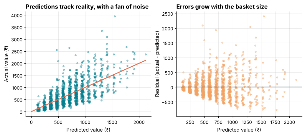

How it works: A residual is actual minus predicted. In the left plot, points on the diagonal are perfect predictions. In the right plot, residuals should look like a patternless band around zero. A funnel shape (errors growing with the prediction) is called heteroscedasticity: the model is less reliable for large baskets. A curve in the residuals would say a straight line is the wrong shape.

Reading the result: The residuals average 4.2 (centred on zero) but spread more as the predicted value grows. A log transform of the target is one remedy to try; the next example tests it.

Example 7: Log-transform the target

Question: Does modelling log(value) fix the widening errors?

y_train_log, y_test_log = np.log(y_train), np.log(y_test)
log_model = LinearRegression().fit(X_train, y_train_log)
pred_log = np.exp(log_model.predict(X_test))

print("R2 on rupees (log model)  :", round(r2_score(y_test, pred_log), 3))
print("MAE on rupees (log model) :", round(mean_absolute_error(y_test, pred_log), 1))
print("MAE on rupees (plain)     :", round(mean_absolute_error(y_test, pred), 1))
print("units coefficient (log)   :", round(log_model.coef_[0], 3), "->", f"{np.exp(log_model.coef_[0]) - 1:.1%} per unit")

R2 on rupees (log model)  : 0.221
MAE on rupees (log model) : 288.8
MAE on rupees (plain)     : 260.0
units coefficient (log)   : 0.182 -> 19.9% per unit

How it works: Predicting log(value) and then exponentiating back turns the model multiplicative: each coefficient becomes "percentage change per unit", and relative errors become more uniform. We always judge the result in the original unit (rupees), so the comparison with the plain model is fair. A log model is not guaranteed to win on every metric; it is a tool for when errors scale with the size of the target.

Reading the result: The log model has MAE ₹289 against ₹260 for the plain model. So on this measure the log model does not win: it describes proportional errors well, but an MAE in rupees is dominated by the large baskets. Each extra unit raises the basket value by about 20%. Always judge a transformation on the metric the business cares about.

Example 8: Categorical features with one-hot encoding

Question: Does the city or delivery slot help predict the order value?

cat = pd.get_dummies(df[["city", "delivery_slot"]], drop_first=True, dtype=int)
X2 = pd.concat([df[features], cat], axis=1)
print("feature count:", X2.shape[1])

X2_train, X2_test, y2_train, y2_test = train_test_split(X2, y, test_size=0.25, random_state=42)
m2 = LinearRegression().fit(X2_train, y2_train)
print("R2 test with city+slot:", round(r2_score(y2_test, m2.predict(X2_test)), 3))
print("R2 test without       :", round(r2_score(y_test, pred), 3))

feature count: 14
R2 test with city+slot: 0.518
R2 test without       : 0.517

How it works: Regression needs numbers, so categories become 0/1 columns, one per category (one-hot encoding). drop_first=True drops one category per variable, which acts as the reference level and avoids redundant columns. Because we used the same random_state, the split is identical, which makes the two R-squared values comparable.

Reading the result: Adding 10 city and slot columns changes the test R-squared by only 0.001: where and when someone orders tells us almost nothing about basket size.

Example 9: Overfitting and cross-validation

Question: Can a more complex model look better on training data and worse on new data?

from sklearn.preprocessing import PolynomialFeatures
from sklearn.pipeline import make_pipeline
from sklearn.model_selection import cross_val_score
import warnings
warnings.filterwarnings("ignore")

results = {}
for degree in (1, 3, 8):
    train_scores, cv_scores = [], []
    for seed in range(30):                      # 30 different small samples of 40 orders
        small = df.sample(40, random_state=seed)
        Xs, ys = small[["units"]], small["value"]
        pipe = make_pipeline(PolynomialFeatures(degree), LinearRegression())
        train_scores.append(pipe.fit(Xs, ys).score(Xs, ys))
        cv_scores.append(cross_val_score(pipe, Xs, ys, cv=5, scoring="r2").mean())
    results[degree] = (np.mean(train_scores), np.median(cv_scores))
    print(f"degree {degree}: train R2 {results[degree][0]:.3f}   cross-validated R2 (median) {results[degree][1]:.3f}")

degree 1: train R2 0.525   cross-validated R2 (median) 0.217
degree 3: train R2 0.572   cross-validated R2 (median) 0.199
degree 8: train R2 0.575   cross-validated R2 (median) -6.796

How it works: A more flexible model (a higher-degree polynomial) always fits the training points at least as well, but it can start memorising noise: that is overfitting. Cross-validation (cross_val_score) repeatedly holds out part of the data, fits on the rest and scores on the held-out part, giving a more honest estimate. To avoid drawing conclusions from one lucky or unlucky sample, we repeat the experiment on 30 different samples of only 40 orders and take the median. Whenever training performance improves while validation performance falls, the model is memorising.

Reading the result: As the degree rises from 1 to 8 the average training R-squared creeps up (0.52 to 0.57), but the median cross-validated R-squared collapses from 0.22 to -6.8. The flexible model looks better on the data it has seen and is far worse on new data.

Example 10: When there is no signal

Question: Can we predict delivery time from order details?

dm = df.dropna(subset=["delivery_minutes"])
Xd = dm[features]
yd = dm["delivery_minutes"]
Xd_train, Xd_test, yd_train, yd_test = train_test_split(Xd, yd, test_size=0.25, random_state=42)

m_d = LinearRegression().fit(Xd_train, yd_train)
pred_d = m_d.predict(Xd_test)
base_d = DummyRegressor().fit(Xd_train, yd_train).predict(Xd_test)

print("R2 test:", round(r2_score(yd_test, pred_d), 4))
print("MAE model   :", round(mean_absolute_error(yd_test, pred_d), 2))
print("MAE baseline:", round(mean_absolute_error(yd_test, base_d), 2))

R2 test: 0.0006
MAE model   : 5.5
MAE baseline: 5.5

How it works: We repeat the same recipe for delivery minutes. When a model has no signal to find, R-squared on the test set sits at or just below zero and the MAE is no better than the baseline. This is an answer, not a failure: the order details we have do not explain delivery time, so we should look for other information (distance, rider availability, traffic, weather) rather than a fancier algorithm.

Reading the result: The test R-squared is 0.001, and the MAE is 5.50 minutes against 5.50 for guessing the average. The model has found essentially nothing.

Common mistakes

1. Evaluating on the training data, which rewards memorisation. Always keep a test set.

2. No baseline. An R-squared of 0.5 or an MAE of ₹200 means nothing until you compare it with predicting the mean.

3. Reading coefficients as causes. They describe association in the data you have.

4. Extrapolating beyond the range of the training data, where a line may not hold.

5. Leaking information: using a feature that would not be known at prediction time (for example, using payment status to predict whether an order is cancelled).

LinearRegression().fit(df[["city"]], df["value"])

Traceback (most recent call last):
  File "example.py", line 1, in <module>
    LinearRegression().fit(df[["city"]], df["value"])
    ~~~~~~~~~~~~~~~~~~~~~~^^^^^^^^^^^^^^^^^^^^^^^^^^^
  File "example.py", line 1403, in wrapper
    return fit_method(estimator, *args, **kwargs)
  File "example.py", line 681, in fit
    X, y = validate_data(
           ~~~~~~~~~~~~~^
        self,
        ^^^^^
    ...<5 lines>...
        force_writeable=True,
        ^^^^^^^^^^^^^^^^^^^^^
    )
    ^
  File "example.py", line 3058, in validate_data
    X, y = check_X_y(X, y, **check_params)
           ~~~~~~~~~^^^^^^^^^^^^^^^^^^^^^^
  File "example.py", line 1330, in check_X_y
    X = check_array(
        X,
    ...<12 lines>...
        input_name="X",
    )
  File "example.py", line 1038, in check_array
    array = _asarray_with_order(array, order=order, dtype=dtype, xp=xp)
  File "example.py", line 983, in _asarray_with_order
    array = numpy.asarray(array, order=order, dtype=dtype)
  File "example.py", line 2027, in __array__
    arr = np.asarray(values, dtype=dtype)
ValueError: could not convert string to float: 'Mumbai'

Practice questions

Practice 1 (Easy): Predict a single basket

Using the model from Example 4, predict the value of an order with 8 units, 5 lines, 0% discount, on a weekday.

new = pd.DataFrame({"units": [8], "lines": [5], "discount_pct": [0], "weekend": [0]})
p8 = model.predict(new)[0]
print(round(p8, 1))

938.1

Practice 2 (Medium): Compare MAE across cities

Using the Example 4 model's test predictions, compute the MAE per city and identify where the model is least accurate.

test_cities = df.loc[X_test.index, "city"]
errors = pd.DataFrame({"city": test_cities, "abs_error": (y_test - pred).abs()})
by_city = errors.groupby("city")["abs_error"].mean().sort_values()
print(by_city.round(1))

city
Kolkata      241.8
Chennai      246.6
Delhi        254.4
Mumbai       255.2
Bengaluru    258.8
Hyderabad    261.6
Ahmedabad    268.7
Pune         302.3
Name: abs_error, dtype: float64

Practice 3 (Hard): Logistic regression for cancellations

Predict whether an order is cancelled from units, lines, discount_pct and weekend using LogisticRegression, and report the test ROC-AUC against the 0.5 you would get by guessing.

from sklearn.linear_model import LogisticRegression
from sklearn.metrics import roc_auc_score

all_orders = orders.merge(basket, on="order_id")
all_orders["weekend"] = (all_orders["order_date"].dt.dayofweek >= 5).astype(int)
all_orders["cancelled"] = (all_orders["order_status"] == "Cancelled").astype(int)

Xc = all_orders[features]
yc = all_orders["cancelled"]
Xc_train, Xc_test, yc_train, yc_test = train_test_split(Xc, yc, test_size=0.25, random_state=42, stratify=yc)

clf = LogisticRegression(max_iter=1000).fit(Xc_train, yc_train)
auc = roc_auc_score(yc_test, clf.predict_proba(Xc_test)[:, 1])
print(round(yc.mean(), 4), round(auc, 3))

0.0617 0.493

Key takeaways

• Regression predicts a numeric target; the slope says how much it changes per unit of a feature.
• The scikit-learn recipe is fit, predict, and score or a metric on held-out data.
• Always split data (or cross-validate), and always compare with a baseline.
• MAE is the typical miss in the target's unit; R-squared compares the model with predicting the mean.
• Plot residuals: curves or funnels show the model is missing something.
• A model with no signal is a result: it tells you to look for better data, not a fancier algorithm.