
Correlation vs Causation: Key Differences, 15 Real Examples and How to Prove Causation
By Skillancy Editorial Team · 21 October 2026 · 22 min read
Reviewed by Rishav Kumar, Principal Data Analyst, Walmart Global Tech
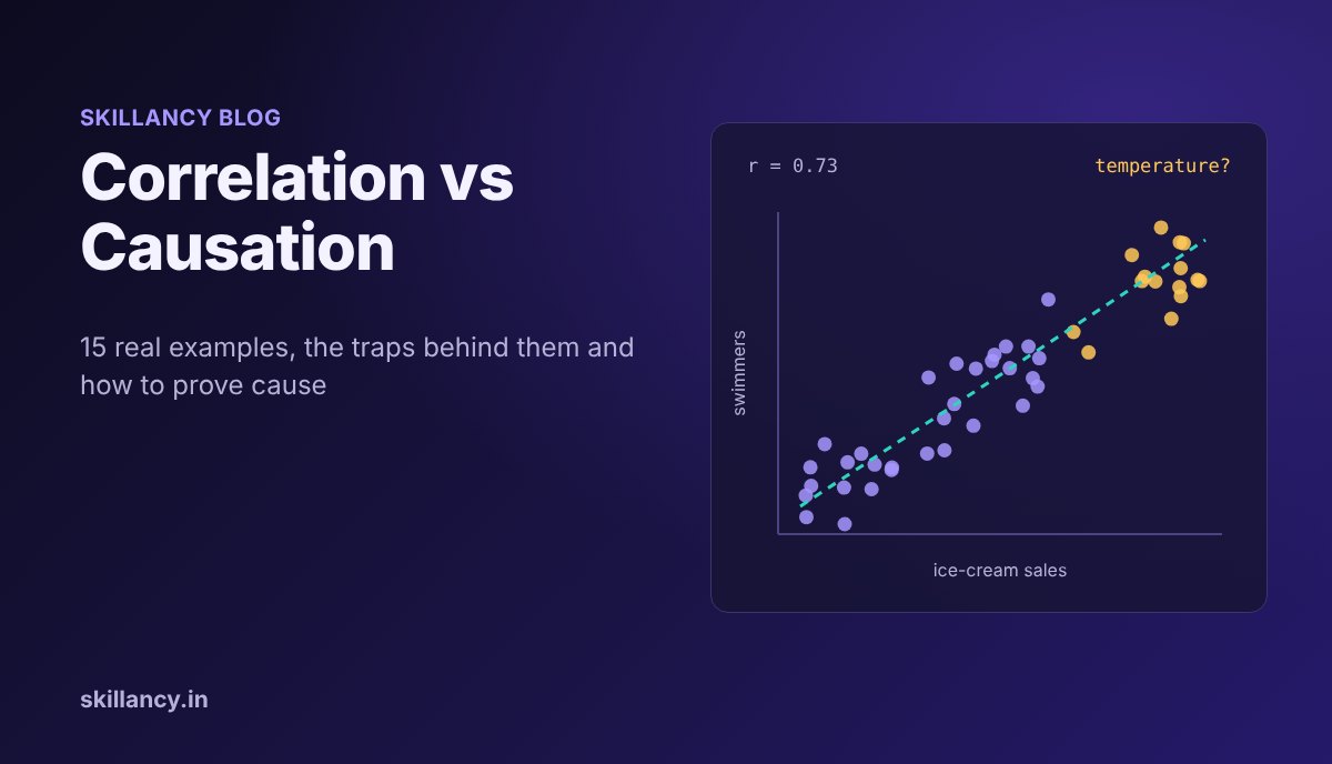
Correlation vs causation is the difference between two things moving together and one thing actually making the other happen. Correlation is a pattern you can measure in any dataset. Causation is a claim about cause and effect, and it needs more evidence than a pattern: usually a controlled experiment, or a study design that rules out every other explanation. This guide explains both ideas in plain language, walks through 15 correlation vs causation examples from everyday life, landmark research and real analyst work, shows the traps in Python with real outputs, and ends with how to prove causation and how to answer the question in an interview.
What is correlation?
Correlation describes how two variables move together. If they rise and fall together, the correlation is positive; if one rises while the other falls, it is negative; if there is no consistent pattern, it is close to zero.
The most common measure is the Pearson correlation coefficient, written r, which runs from −1 to +1:
| Value of r | What it means | Example |
|---|---|---|
| +1 | Perfect positive linear relationship | Distance driven and fuel used at constant speed |
| +0.5 to +0.9 | Moderate to strong positive | Hours studied and test score |
| Around 0 | No linear relationship | Shoe size and salary |
| −0.5 to −0.9 | Moderate to strong negative | Price of a product and units sold |
| −1 | Perfect negative linear relationship | Battery remaining and minutes of use at a fixed drain |
Pearson's r captures straight-line relationships. Spearman's rank correlation works on ranks instead, so it also catches relationships that always go up (or down) but not in a straight line, and it is less affected by outliers. Either way, a correlation coefficient only summarizes a pattern. It says nothing about why the pattern exists.
What is causation?
Causation (also called causality or a causal relationship) means that changing one variable, the cause, produces a change in another, the effect, with everything else held the same. Pressing the brake causes a car to slow down. A price cut causes more units to sell. The test of causation is a counterfactual question: if we had changed X and nothing else, would Y have been different?
That "nothing else" is the hard part. In real data, many things change at once, which is why correlation is easy to find and causation is hard to prove.
Correlation vs causation: the key differences
| Aspect | Correlation | Causation |
|---|---|---|
| What it says | X and Y move together | Changing X changes Y |
| Direction | Symmetric: X with Y is the same as Y with X | Has a direction: X causes Y, not the reverse |
| How you find it | Calculate a coefficient on existing data | Run an experiment or a design that rules out other explanations |
| Typical evidence | Scatter plot, r, a dashboard trend | A/B test, randomized trial, natural experiment |
| Can it be wrong? | The number is rarely wrong; the interpretation often is | Can be wrong if the design has a flaw |
| Useful for | Prediction, spotting where to look | Decisions and interventions: what happens if we act |
A useful way to remember it: every causal relationship produces a correlation (in the right data), but most correlations are not causal relationships.
Why correlation does not imply causation
When you see two variables moving together, there are at least seven explanations other than "X causes Y". Every example later in this guide is one of these.
| Trap | What is happening | Classic sign |
|---|---|---|
| Confounding (third variable) | A hidden factor Z drives both X and Y | Both variables follow the same season, size or wealth pattern |
| Reverse causation | Y actually causes X | The "effect" could plausibly come first |
| Selection bias (self-selection) | The people who chose X were already different | You compare users who opted in with those who did not |
| Chance and data dredging | You tested so many pairs that some line up by luck | No plausible mechanism, short time series |
| Simpson's paradox | A trend in the total reverses inside groups | Group sizes differ a lot between categories |
| Collider bias | You only looked at cases filtered by both variables | Data restricted to "hired", "admitted", "survived" |
| Regression to the mean | Extreme values naturally drift back toward average | You intervened only on the best or worst performers |
The first three cause most real-world mistakes. Ask about them every time you see a correlation in a report.
15 correlation vs causation examples
Examples 1 to 7 are classics from everyday life and published research. Examples 8 to 15 are the kind of patterns analysts meet in business data; they describe common situations rather than findings from one specific company.
| # | Correlation observed | Main trap |
|---|---|---|
| 1 | Ice-cream sales and drownings | Confounding (hot weather) |
| 2 | More firefighters, more fire damage | Confounding (size of the fire) |
| 3 | Storks and birth rates in Europe | Confounding (country size) |
| 4 | Chocolate and Nobel prizes | Confounding (national wealth), ecological data |
| 5 | Hormone therapy and heart disease | Healthy-user selection |
| 6 | Berkeley admissions and gender | Simpson's paradox |
| 7 | Nicolas Cage films and pool drownings | Pure chance |
| 8 | Coupon users spend more | Selection bias |
| 9 | Push-notification users retain better | Self-selection |
| 10 | Ad spend and festive-season sales | Confounding (season) and reverse causation |
| 11 | Support tickets and churn | Common cause (product problems) |
| 12 | Training attendance and promotions | Selection bias |
| 13 | More delivery riders, slower deliveries | Reverse causation |
| 14 | New managers turn around the worst stores | Regression to the mean |
| 15 | Hired analysts with great SQL seem weaker communicators | Collider bias |
Example 1: Ice-cream sales and drownings
The correlation: On days when more ice cream is sold, more people drown.
What is really going on: Hot weather. On hot days people buy ice cream, and far more people go swimming, which raises the number of drownings. Temperature is a confounder: it causes both variables. Ice cream does not cause drowning, and banning it would save no one.
How to check: Compare days with the same temperature. Within a narrow temperature band, the link between ice cream and drownings largely disappears. You can see exactly this in the Python demo later in this guide.
Example 2: More firefighters, more fire damage
The correlation: Fires attended by more firefighters cause more damage.
What is really going on: Bigger fires get more firefighters, and bigger fires cause more damage. The size of the fire drives both. Concluding that firefighters cause damage gets the story backwards and would lead to a disastrous policy.
How to check: Compare fires of similar size and type. Holding fire size fixed, more firefighters is associated with less damage, which is what you would expect.
Example 3: Storks and birth rates
The correlation: In a 2000 paper titled "Storks Deliver Babies (p = 0.008)" in Teaching Statistics, Robert Matthews showed that across 17 European countries, the number of breeding stork pairs predicted the birth rate, with a statistically significant result.
What is really going on: Country size. Larger countries have more land for storks and more people having babies. When land area is added to the model, the stork effect stops being significant. Matthews wrote the paper deliberately to show that a small p-value does not prove causation.
How to check: Adjust for the obvious size variable (land area or population) before reading anything into a cross-country correlation.
Example 4: Chocolate consumption and Nobel prizes
The correlation: A 2012 note by Franz Messerli in the New England Journal of Medicine reported a correlation of r = 0.791 across 23 countries between chocolate eaten per person and Nobel laureates per 10 million people.
What is really going on: Wealthy countries can afford both more chocolate and well-funded universities and research systems. National wealth is a plausible confounder. The data is also ecological: it compares country averages, so it says nothing about whether any individual who eats chocolate becomes a better scientist.
How to check: Control for GDP per capita and research spending, and never jump from country-level averages to claims about individuals.
Example 5: Hormone therapy and heart disease
The correlation: For years, observational studies found that postmenopausal women who took hormone replacement therapy (HRT) had lower rates of heart disease, and many doctors recommended it partly for that reason.
What is really going on: The randomized Women's Health Initiative trial tested it directly. Its estrogen-plus-progestin arm, with 16,608 women, was stopped early in 2002 after a mean follow-up of 5.2 years. Instead of protection, women on the therapy had a higher risk of coronary heart disease (hazard ratio 1.29), stroke (1.41) and invasive breast cancer (1.26) than women on placebo. A widely discussed explanation for the earlier observational results is that women who chose hormone therapy differed from those who did not in ways that also protect the heart, often called the healthy-user effect.
How to check: This is the textbook case for why randomization matters. When people choose the treatment themselves, you are partly measuring who chooses it.
Example 6: Berkeley graduate admissions and gender
The correlation: In fall 1973, the University of California, Berkeley admitted about 44% of 8,442 male applicants to its graduate programs but only about 35% of 4,321 female applicants. It looked like clear evidence of bias against women.
What is really going on: When Bickel, Hammel and O'Connell analysed the data department by department (Science, 1975), most departments showed no significant bias, and about as many favored women as favored men. Women had applied more often to highly competitive departments that rejected most applicants of either gender, which pulled down their overall rate. This reversal between the total and the groups is Simpson's paradox. The Python demo below reproduces it with the six largest departments.
How to check: Whenever group sizes differ a lot, break the total down by the most relevant grouping before drawing a conclusion.
Example 7: Nicolas Cage films and swimming-pool drownings
The correlation: Tyler Vigen's well-known "spurious correlations" collection shows that the number of films Nicolas Cage appeared in each year tracked the number of people who drowned by falling into a swimming pool in the United States over the same years.
What is really going on: Nothing. With thousands of yearly statistics available, some pairs will line up by coincidence, especially over a short run of years. This is chance plus data dredging: search enough pairs and you are guaranteed to find impressive-looking matches.
How to check: Ask for a plausible mechanism, test the pattern on new data it was not discovered in, and be very suspicious of short time series that happen to match.
Example 8: Customers who use coupons spend more
The correlation: In an e-commerce dashboard, customers who used a discount coupon spend far more per month than customers who did not. A manager proposes sending coupons to everyone to raise spending.
What is really going on: Keen, high-intent customers are the ones who go looking for coupons. They would have spent more anyway. This is selection bias: the coupon group and the no-coupon group were different before any coupon was used. The true effect of a coupon might be small, zero, or even negative once you count the discount cost.
How to check: Run an A/B test: send the coupon to a random half of customers and compare spending against the other half. The demo below shows how badly the naive comparison can overstate the effect.
Example 9: Users who enable push notifications retain better
The correlation: In a mobile app, users who turned on push notifications have much higher 90-day retention than users who did not.
What is really going on: Users who are already engaged and plan to keep using the app are more likely to accept notifications. Turning on notifications may help a little, but the gap mostly reflects who opts in (self-selection). Forcing the permission prompt on everyone will not reproduce the gap.
How to check: Randomize the prompt itself: show a notification permission prompt to a random group at a given point, and compare retention between the groups that were and were not prompted, regardless of whether individuals accepted.
Example 10: Ad spend and festive-season sales
The correlation: Monthly ad spend and sales rise and fall together, with both peaking around Diwali and other festive months.
What is really going on: Two things. The festive season drives demand regardless of advertising (confounding by seasonality), and marketing teams set bigger budgets for the months they already expect to sell more (reverse causation: expected sales drive ad spend). A simple correlation between monthly spend and sales overstates what advertising adds.
How to check: Use geo experiments (turn ads up or off in randomly chosen cities or regions), holdout groups, or at least compare year-on-year for the same festive weeks with different spend levels.
Example 11: Support tickets and churn
The correlation: Customers who raised more support tickets are more likely to cancel their subscription.
What is really going on: Product problems cause both the tickets and the churn. Contacting support is a symptom, not the cause. Making support harder to reach would hide the symptom and probably increase churn. The right reading is that tickets are a useful warning signal for churn prediction, not a lever to cut.
How to check: Separate prediction from intervention. Use tickets as a feature in a churn model, but test changes to support (faster responses, proactive fixes) with a randomized rollout.
Example 12: Training attendance and promotions
The correlation: Employees who attended an optional leadership programme were promoted at twice the rate of those who did not.
What is really going on: Ambitious, high-performing employees, often nominated by their managers, are the ones who sign up. They were more likely to be promoted with or without the programme (selection bias).
How to check: If seats are limited, allocate them by lottery among volunteers and compare winners with non-winners. Failing that, compare against similar employees with matching ratings and tenure, and be honest that the result is weaker evidence.
Example 13: More delivery riders, slower deliveries
The correlation: In a food-delivery dataset, hours with more delivery partners online also have longer average delivery times.
What is really going on: Reverse causation. Operations teams and incentive schemes bring more riders online precisely when demand surges, such as dinner peaks, rain or match nights, and those are also the hours when restaurants and roads are slowest. Demand drives both rider supply and delivery time. Removing riders would make deliveries slower, not faster.
How to check: Compare hours with similar order volume, weather and traffic, or analyse the effect of a supply change you did not cause yourself, such as an unplanned app outage on the rider side.
Example 14: New managers turn around the worst stores
The correlation: A retailer moved new managers into its 20 worst-performing stores last quarter. This quarter, those stores improved sharply, and the new managers are credited.
What is really going on: Some of the improvement is probably regression to the mean. A store that had an unusually bad quarter, from a local disruption, a supply problem or plain bad luck, tends to move back toward its normal level the next quarter without any intervention. Picking stores because they were extreme guarantees some bounce-back.
How to check: Compare against a control group: other stores that were just as bad last quarter but did not get a new manager. Only the improvement beyond theirs can be credited to the change.
Example 15: Hired analysts with great SQL seem to be weaker communicators
The correlation: Looking only at analysts the team hired, the ones with the strongest SQL scores seem to have weaker communication skills, and someone concludes the two skills trade off.
What is really going on: Collider bias (also called Berkson's paradox). Candidates got hired if their overall profile was strong enough, so a hired candidate with average SQL must have been strong on communication, and vice versa. Filtering on an outcome that both skills contribute to creates a negative correlation inside the filtered group, even if the skills are unrelated, or positively related, among all applicants.
How to check: Look at the full applicant pool, not only the people who passed the filter. Be careful whenever your data only contains people who were hired, admitted, approved or survived.
See it in Python: three traps with real outputs
You can run these snippets in the free Skillancy Python compiler. The outputs below were produced with pandas 3.
1. A confounder creates a strong correlation
Here temperature drives both ice-cream sales and the number of swimmers, and nothing else connects them:
import numpy as np
import pandas as pd

rng = np.random.default_rng(7)
days = 365
temp = rng.normal(30, 5, days).round(1)                          # daily max temperature, °C
ice_cream = (50 + 12 * temp + rng.normal(0, 30, days)).round()   # cones sold
swimmers = (20 + 6 * temp + rng.normal(0, 20, days)).round()     # people at the beach

df = pd.DataFrame({"temp": temp, "ice_cream": ice_cream, "swimmers": swimmers})
print(df[["ice_cream", "swimmers"]].corr().round(2))

def residuals(y, x):
    slope, intercept = np.polyfit(x, y, 1)
    return y - (slope * x + intercept)

r_partial = np.corrcoef(residuals(df["ice_cream"], df["temp"]),
                        residuals(df["swimmers"], df["temp"]))[0, 1]
print(round(r_partial, 2))
Output:
           ice_cream  swimmers
ice_cream       1.00      0.73
swimmers        0.73      1.00
0.02
The raw correlation is a strong 0.73. The second number is the partial correlation: the correlation left over after removing the part of each variable that temperature explains. It drops to 0.02, essentially zero, because temperature was the whole story.
2. Simpson's paradox with the Berkeley data
These are the admission counts for the six largest departments in the 1973 Berkeley data, the same figures used in R's built-in UCBAdmissions dataset:
import pandas as pd

berkeley = pd.DataFrame({
    "dept":     list("ABCDEF") * 2,
    "gender":   ["Men"] * 6 + ["Women"] * 6,
    "applied":  [825, 560, 325, 417, 191, 373, 108, 25, 593, 375, 393, 341],
    "admitted": [512, 353, 120, 138, 53, 22, 89, 17, 202, 131, 94, 24],
})

overall = berkeley.groupby("gender")[["applied", "admitted"]].sum()
overall["rate_%"] = (100 * overall["admitted"] / overall["applied"]).round(1)
print(overall)

by_dept = berkeley.assign(rate=(100 * berkeley["admitted"] / berkeley["applied"]).round(1))
print(by_dept.pivot(index="dept", columns="gender", values="rate"))
Output:
        applied  admitted  rate_%
gender
Men        2691      1198    44.5
Women      1835       557    30.4
gender   Men  Women
dept
A       62.1   82.4
B       63.0   68.0
C       36.9   34.1
D       33.1   34.9
E       27.7   23.9
F        5.9    7.0
Overall, men were admitted at 44.5% and women at 30.4%. Department by department, women had a higher admission rate in four of the six. The reversal happens because most women applied to departments C to F, which admitted few applicants of either gender, while most men applied to A and B, which admitted most applicants.
3. Why A/B tests beat observational comparisons
This simulation builds in a true coupon effect of exactly ₹50 of extra spend, plus a hidden "intent" variable that makes keen customers both spend more and seek out coupons:
import numpy as np
import pandas as pd

rng = np.random.default_rng(42)
n = 20_000
intent = rng.normal(0, 1, n)                       # how keen the customer already is (unobserved)

# Observational world: keen customers go looking for coupons
used_coupon = rng.random(n) < 1 / (1 + np.exp(-1.5 * intent))
spend = 1000 + 400 * intent + 50 * used_coupon + rng.normal(0, 200, n)
obs = pd.DataFrame({"coupon": used_coupon, "spend": spend})
print(obs.groupby("coupon")["spend"].mean().round(0))

# Experiment: coupons sent at random, so intent is balanced across groups
sent_coupon = rng.random(n) < 0.5
spend_ab = 1000 + 400 * intent + 50 * sent_coupon + rng.normal(0, 200, n)
ab = pd.DataFrame({"coupon": sent_coupon, "spend": spend_ab})
print(ab.groupby("coupon")["spend"].mean().round(0))
Output:
coupon
False     783.0
True     1263.0
Name: spend, dtype: float64
coupon
False     999.0
True     1050.0
Name: spend, dtype: float64
The observational comparison says coupon users spend ₹480 more, almost ten times the real effect. The randomized comparison finds ₹51, very close to the true ₹50. Randomization works because it makes the two groups alike in everything, including the variables you never measured. For a full significance test on an A/B result, see the A/B test section of our Python for data science guide.
How to establish causation
There is no single formula, but there is a clear order of strength.
| Method | How it works | When to use it |
|---|---|---|
| Randomized controlled trial / A/B test | Randomly assign the treatment, compare outcomes | Whenever you control the intervention and it is ethical |
| Natural experiment | Use an event that assigned treatment "as if" randomly | Policy changes, outages, lotteries, cut-off dates |
| Difference-in-differences | Compare the before-after change in a treated group with the change in a similar untreated group | Rollouts by city, store or region |
| Regression discontinuity | Compare cases just above and below a threshold | Eligibility cut-offs, score thresholds |
| Instrumental variables | Use a factor that affects the treatment but not the outcome directly | When a good instrument exists, which is rare |
| Regression with controls / matching | Adjust for measured confounders | Only when experiments are impossible; cannot fix unmeasured confounders |
When you cannot experiment, epidemiologists still use the nine viewpoints Sir Austin Bradford Hill proposed in 1965 in "The Environment and Disease: Association or Causation?". They are a checklist for judging whether an association is likely to be causal, not a proof:
1. Strength: a large association is harder to explain away.
2. Consistency: the result repeats across studies, places and people.
3. Specificity: the cause is linked to a specific effect.
4. Temporality: the cause comes before the effect. This one is essential.
5. Biological gradient (dose-response): more of the cause leads to more of the effect.
6. Plausibility: there is a believable mechanism.
7. Coherence: the claim fits what is already known.
8. Experiment: changing the cause changes the effect.
9. Analogy: similar causes are known to have similar effects.
Smoking and lung cancer is the famous case where these criteria, applied to decades of observational evidence, built a convincing causal argument without a randomized trial on humans.
A five-question checklist before you claim causation
Use this on any dashboard insight before it goes into a deck:
1. Could a third factor drive both? Think season, size, wealth, intent, demand, age.
2. Could the arrow point the other way? Does Y plausibly cause X?
3. Who chose to be in each group? If people opted in, you are partly measuring who opts in.
4. Was the data filtered? Only customers who converted, only hired candidates, only surviving stores.
5. Would it hold on new data or in an experiment? If you can test it, test it.
If you cannot rule these out, the honest wording is "is associated with", not "causes", "drives" or "leads to".
How to answer "correlation vs causation" in an interview
This is one of the most common statistics questions in data analyst interviews, and it often comes up again inside a case question. A strong answer has four parts: a definition, an example, the reason, and how you would test it.
"Correlation means two metrics move together; causation means changing one actually changes the other. For example, ice-cream sales and drownings are correlated because hot weather drives both, not because one causes the other. Correlation can come from a confounder, reverse causation, selection bias or chance. To show causation I would run an A/B test, or, if that is not possible, use something like difference-in-differences with a comparable control group and check that the cause comes before the effect."
Then apply it to the business. If the interviewer says "users who use feature X retain better, should we push everyone to use it?", say that the users may have self-selected, and propose a randomized rollout or an encouragement test before investing. For more questions like this, see our guide to data analyst interview questions.
Practise this answer out loud before the real thing. Book a mock interview with a practitioner who hires analysts and get feedback on how you explain statistics, SQL and case questions.
Common mistakes analysts make
- Writing "drives" or "leads to" in a report when the analysis only shows a correlation.
- Treating a small p-value as proof of causation. The stork paper had p = 0.008.
- Comparing opt-in users with everyone else and calling the difference the feature's impact.
- Ignoring time order: checking whether the supposed cause came first is the cheapest test there is.
- Adding every available control variable to a regression. Controlling for a variable caused by the treatment, or for a collider, can create bias instead of removing it.
- Concluding there is no relationship because r is near zero. Pearson's r only measures straight-line relationships; a strong curved relationship can still have r close to 0. Always plot the data.
Frequently asked questions
What is the difference between correlation and causation?
Correlation means two variables change together. Causation means a change in one variable produces a change in the other. Correlation can be calculated from any dataset; causation needs evidence that rules out other explanations, usually an experiment.
Why does correlation not imply causation?
Because the same pattern can be produced by a third variable that drives both, by the effect running in the opposite direction, by how the data was selected, or by coincidence. A correlation alone cannot tell these apart from a true cause.
What is a simple example of correlation vs causation?
Ice-cream sales and drownings rise together, but hot weather causes both. Ice cream does not cause drowning, so the relationship is a correlation without causation.
Can correlation ever prove causation?
Not on its own. A correlation becomes strong evidence of causation only when it comes from a randomized experiment or a design that rules out confounding, and when it fits criteria such as the cause coming before the effect and a dose-response pattern.
What is a confounding variable?
A confounder is a third variable that influences both the supposed cause and the effect, creating a correlation between them. Temperature is the confounder in the ice-cream and drowning example; country size is the confounder in the storks and babies example.
How do you test for causation in data analytics?
The strongest method is an A/B test, where users are randomly split and only one group gets the change. When that is not possible, analysts use natural experiments, difference-in-differences, regression discontinuity or carefully controlled regression, and state the limitations clearly.
What is the difference between correlation and regression?
Correlation measures the strength and direction of a relationship with one number. Regression models how one variable changes with one or more others and can adjust for measured confounders. Neither proves causation by itself; that depends on how the data was generated.
Is correlation vs causation asked in data analyst interviews?
Yes. It is one of the most common statistics questions for analyst roles in India, and it often reappears inside case questions about why a metric changed or whether a feature caused an improvement.
Recommended internal links
- Data analyst interview questions with model answers: https://skillancy.in/blog/data-analyst-interview-questions
- Python for data science, including an A/B test: https://skillancy.in/blog/python-for-data-science
- Free online Python compiler: https://skillancy.in/tools/python-compiler
- Python interview questions with a live editor: https://skillancy.in/practice/python-questions
- Data Analytics with Agentic AI program: https://skillancy.in/courses/data-analytics-with-agentic-ai
- Data Science with AI program: https://skillancy.in/courses/data-science-with-ai
Sources and publishing references
Bickel, Hammel and O'Connell, "Sex Bias in Graduate Admissions: Data from Berkeley", Science, 1975: https://homepage.stat.uiowa.edu/~mbognar/1030/Bickel-Berkeley.pdf
Messerli, chocolate consumption and Nobel laureates (NEJM, 2012), summary on NEJM CardioExchange: https://blogs.nejm.org/cardioexchange/2012/10/10/chocolate-and-nobel-prizes-linked/
Women's Health Initiative estrogen plus progestin trial (JAMA, 2002): https://jamanetwork.com/journals/jama/fullarticle/195120
NHLBI: Women's Health Initiative: https://www.nhlbi.nih.gov/science/womens-health-initiative-whi
Matthews, "Storks Deliver Babies (p = 0.008)", Teaching Statistics, 2000, summarized by De Econometrist: https://www.deeconometrist.nl/article/do-storks-deliver-babies
Bradford Hill criteria (Proceedings of the Royal Society of Medicine, 1965): https://en.wikipedia.org/wiki/Bradford_Hill_criteria
ANU Systems Toolkit: Correlation and causation, including spurious correlations: https://users.cecs.anu.edu.au/~Chris.Browne/systems_toolkit/060_data_analysis/correlation_and_causation/
All Python outputs on this page were produced by running the snippets with NumPy and pandas 3. The simulated datasets use fixed random seeds, so you will get the same numbers.
Get the Skillancy field notes
One email a week: AI and analytics guides, cohort dates and hiring signals. No spam, unsubscribe anytime.